Entity Resolution in Reagent

NOTE 1: This Blog Post is split into two parts. The first is a less technical discussion of how Margin Research’s Reagent Tool works, as well as some awesome results it can produce. The second part is a more technical discussion of AI/ML pipeline technology we integrated.

NOTE 2: Viewing the Linux Kernel Graph. Reagent has ingested tens of thousands of git repositories, but for the sake of simplicity we will generally only view the graph revolving around the Linux Kernel in this discussion. This is also helpful in Part II of the blog post where it is used for ML purposes.

The Margin Research team has been developing under a DARPA funded exploratory program called Social Cyber. Our project under this program is called Reagent. With Reagent, we’ve been doing some very exciting work on the fringes of computer science. Recently, we’ve combined three powerful technologies in novel ways to produce limited but real results, with more to come in the future. The three technologies used are:

1. Graph Databases
2. LLMs (like ChatGPT)
3. AI/ML pipelines
   

First we’ll cover what Reagent does, how it is hosted, and what questions it can answer. We’ll talk about the introduction of LLMs to help build and classify our DB. Then, In Part II we’ll dive into how we’ve integrated machine learning to Reagent to produce small but exciting results.

PT I: What is Reagent?

Reagent bridges the gap between code and people by focusing on the social networks that power Open Source projects. An easier way to say that might be: “We look at a lot of developer and git metadata” That of course is an oversimplification, but it is a key component of how the Margin Research team is able to extract real, valuable insights from our tool. By understanding how developers work, many insights can be surfaced about Open Source itself. Refer to other articles here and here to see some!

In order to capture these social networks, Margin Research relies on neo4j graph databases to host the Reagent tool. A graph database is similar to a traditional database, but uses nodes (entities), edges (relationships), and properties (any additional details) to store information. The huge advantage here over a regular database are the relationships between entities. This is also what makes graph databases so great for social network modeling - they naturally form graphs that resemble networks of people. Below in Figure 1 is a simplified schema for our database, where the circles are node types with lines as relationships between them:

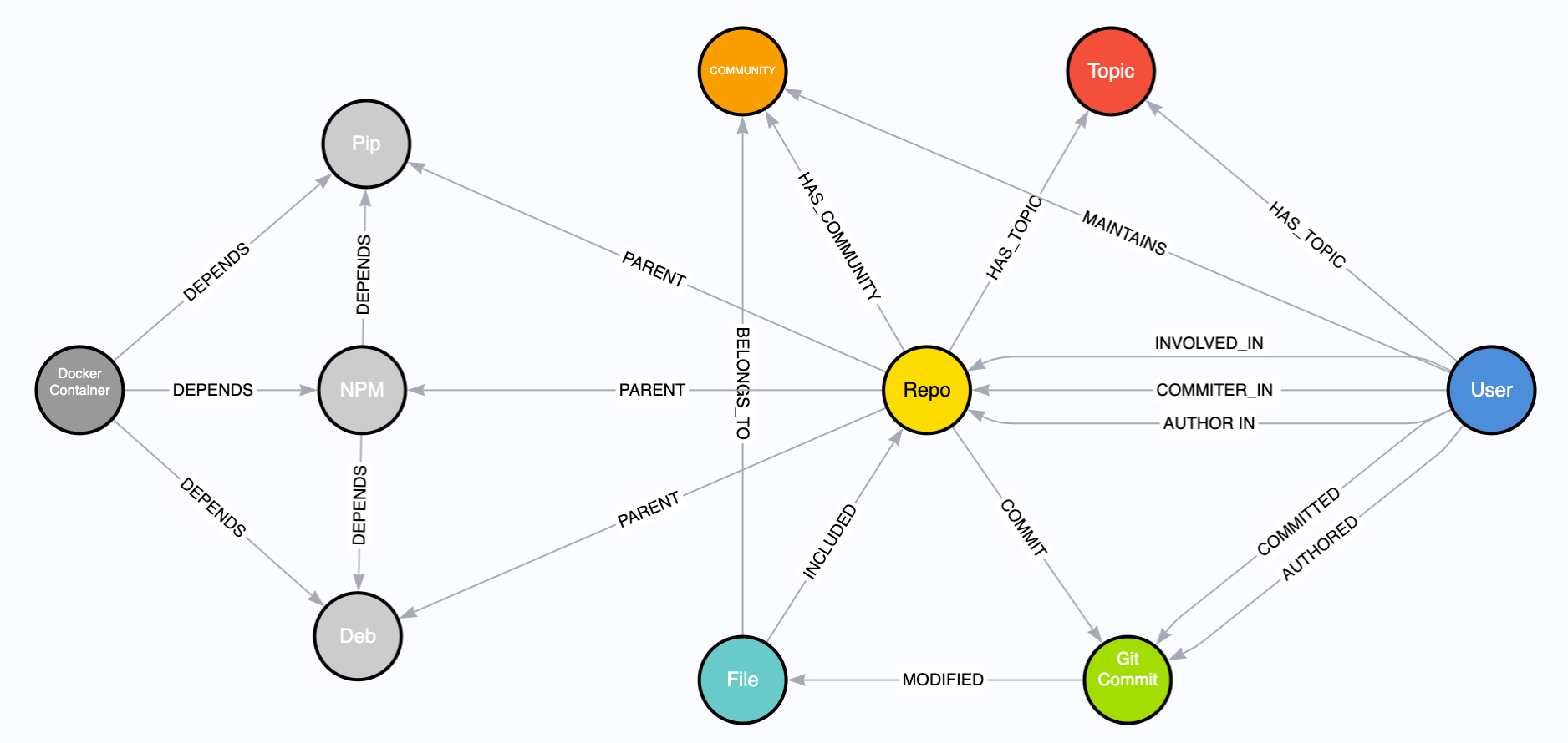
The graph schema is rather intuitive. Users COMMIT_IN Repos which INCLUDE Files. Figure 2 below is an example query and result from our database. This query answers the question: Who contributes to the Linux Kernel?

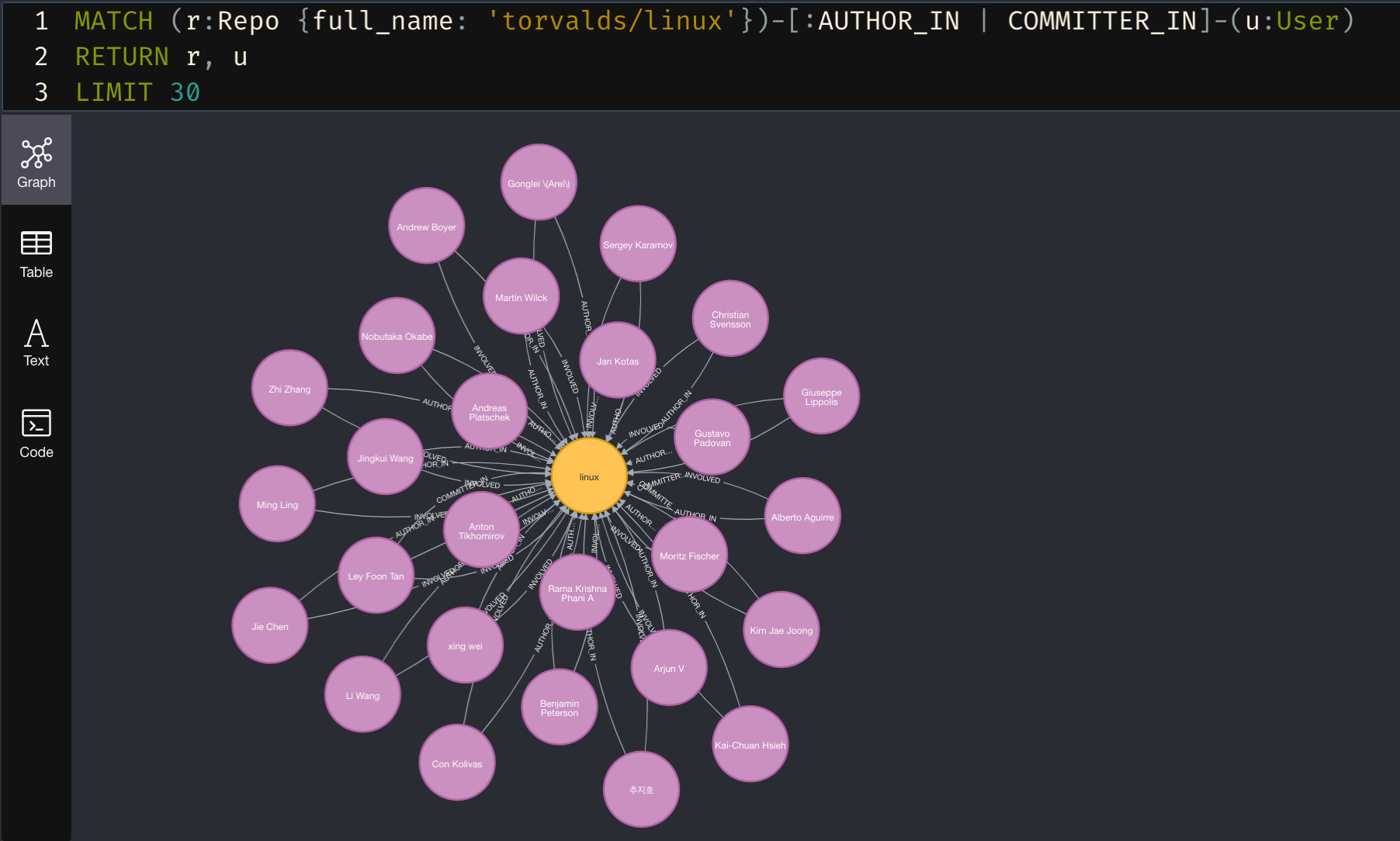
The response here is limited to 30 nodes, while in reality there are many more. It shows Users in pink, who have an AUTHOR_IN or COMMITTER_IN relationship to the Linux Repo node. When combined with the additional node properties, we can filter this query to only view contributors with email addresses from google, or intel, we can find power contributors who have reached a certain threshold of commits, or we can execute graph algorithms such as page rank, k-nearest-neighbor, or Jaccardian distance to do community detection and produce other data enrichments. These enrichments often reveal to us who actually maintains a region of code (hint: it’s often different than the listed maintainer).

One of the immediately valuable aspects of this technology is being able to gather information across different projects and industries. In Figure 3 we adjust the query to answer the question: Which Linux contributors also contribute to BitCoin?

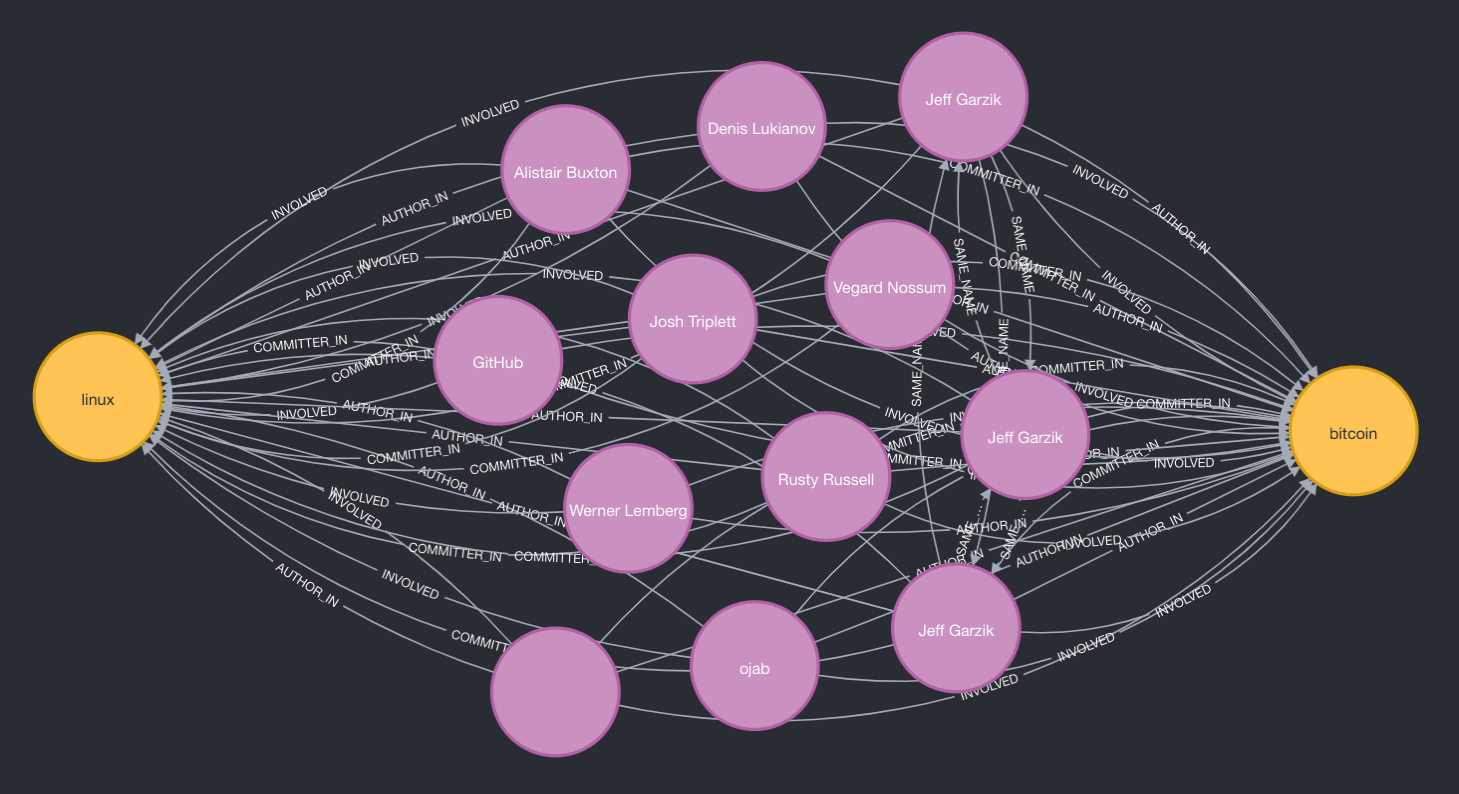
When we think about ingesting tens of thousands of GitHub (and other git) repositories, one can start to understand the power of knowing who is contributing where. It might be useful to know which contributors to a sanctioned cyber security entity, like Positive Technologies, are also committing to the Linux Kernel. Our techniques also allow us to see a project’s health, which is fundamental for security and longevity. Lastly, our graph’s capture project dependencies, so we can see when a popular project depends on smaller, riskier, or unmaintained projects.

The two queries listed above are rather simple. Let's move on to a more complex and valuable question: Who in China works in the Artificial Intelligence Field? Before diving into our answer, it might be helpful to think about how one might try and answer this question. You could google search and comb through research papers. Or you could look at Chinese businesses that market for AI and scrape their staff. Both of these solutions would produce meager results, only capturing a tiny snapshot of the relevant players. We’re rather proud to say that Reagent quickly produces an in-depth answer to this complex question, and allows for analysis and insights past that.

To surface an answer, our tool makes use of the latest LLM APIs to produce “topics” that classify a user's work. These topics are essentially hashtags, but we’ll generally refrain from that term. This itself is a novel usage of AI for data classification which makes large swaths of intractable data searchable. We use this technique to classify GitHub repositories and users by their areas of work. An example Repo’s topics might be: #bitcoin #blockchain #cryptocurrency #crypto #transaction #security #transactionfee #rpc #command #api. Now when we search our DB for #cryptocurrency, the previously unclassified Repo node will be returned!

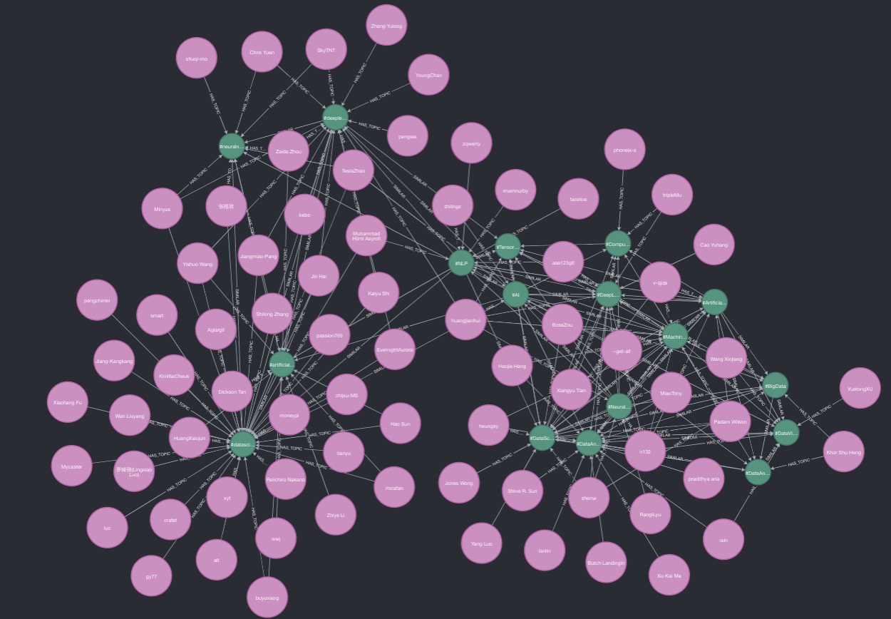
Below is our query and results to answer the previously mentioned question, Who in China works in the Artificial Intelligence Field? Figure 2 below is the query we use. We grab the two Topic nodes that are named: #AI, #ML, and any Topic nodes that have a :SIMILAR relationship to these two keystone nodes. We set a similarity threshold of 0.1. Lastly, we add in any users with timezone = 8 (China) that are attached to these Topic nodes

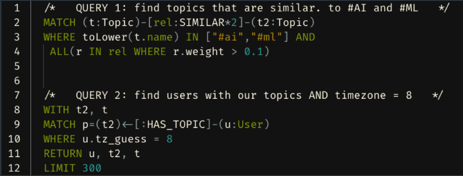
Figure 3 below is the response to our question. We limit our response to 300 nodes. In green are the topics that are originally produced by our LLM tagging technique. We capture tags such as #AI, which was explicitly mentioned, and tags that are similar, such as #DataScience, #NLP, #TensorFlow, #DeepLearning, and many more. Attached to these nodes are the Users with timezone 8 (China), in pink.

At this point it should be clear just how powerful Reagent is.

PT II: Entity Resolution using an AI/ML pipeline in Neo4j with String and Graph Embeddings

(NOTE: This portion of the blog post is more technical than the previous overview of Reagent. We assume the reader has a working knowledge of AI/ML technologies such as embeddings, and a deeper understanding of graph databases than what was presented above.)

One of the biggest challenges in our graph database, and indeed in many modern technologies, is called entity resolution (ER). Entity Resolution is the practice of figuring out when two separate entities are actually the same thing. Here are two examples:

1. A computer, an iphone, and a smart TV are all separate entities that can be condensed down to one entity: the person who is the owner of all three. An ad agency might try to use IP addresses, geolocation, consumer data, and social profiles to figure out that all three of these devices are owned by the same person, and therefore can be served related ads.
2. Multiple contributors to an Open Source project have similar names, emails, and commit histories. The various contributors are originally separate entities defined by email addresses, but with some work, one could figure out that: [email protected], [email protected], and [email protected] are all the same entity: Linus Torvalds.
   

In fact, the second example is exactly what we attempt to do in our graph database. The majority of User nodes we have in our DB are GitHub users. Oftentimes, developers have various GitHub accounts: work, personal, school. But they may contribute to the same projects from these accounts. It’s useful to have three separate User nodes to preserve the clarity of which account contributed what, but it’s extremely powerful to also have a Person node that is related to all three Users. This also allows for deduplication (aka dedup-ing) which is extremely important in many data science projects, including ours.

Applying AI/ML to entity resolution work is itself not novel. In fact, Neo4j has a whole graph data science library that attempts to make this process easy (hint: it’s never easy. ER is hard). Our approach is original due to a two main reasons:

1. Our application of this problem to GitHub contributors, across separate projects
2. Our usage of AI generated topics to create both graph structure and string embeddings, which are fed into the ML pipeline and contribute to the solution to this problem

Before jumping into the technical discussion, it’s important to understand one and two above.

One: After many hours of research (read: banging our heads against computers) we can confidently conclude that nobody else is publicly trying to do ER on GitHub users across separate projects. In fact, nobody is trying to do ER on GitHub users at all. It would be easier to do ER and just focus on one project (who contributes to the Linux Kernel and is actually the same person) but it’s really important to look across projects and see who is contributing to the Linux kernel and is using a different email to contribute offensive security work for a Russian Hacking firm. Sounds like a recipe for a malicious backdoor in the foundational technology of the internet. That of course is just one example of the kinds of problems we think about.

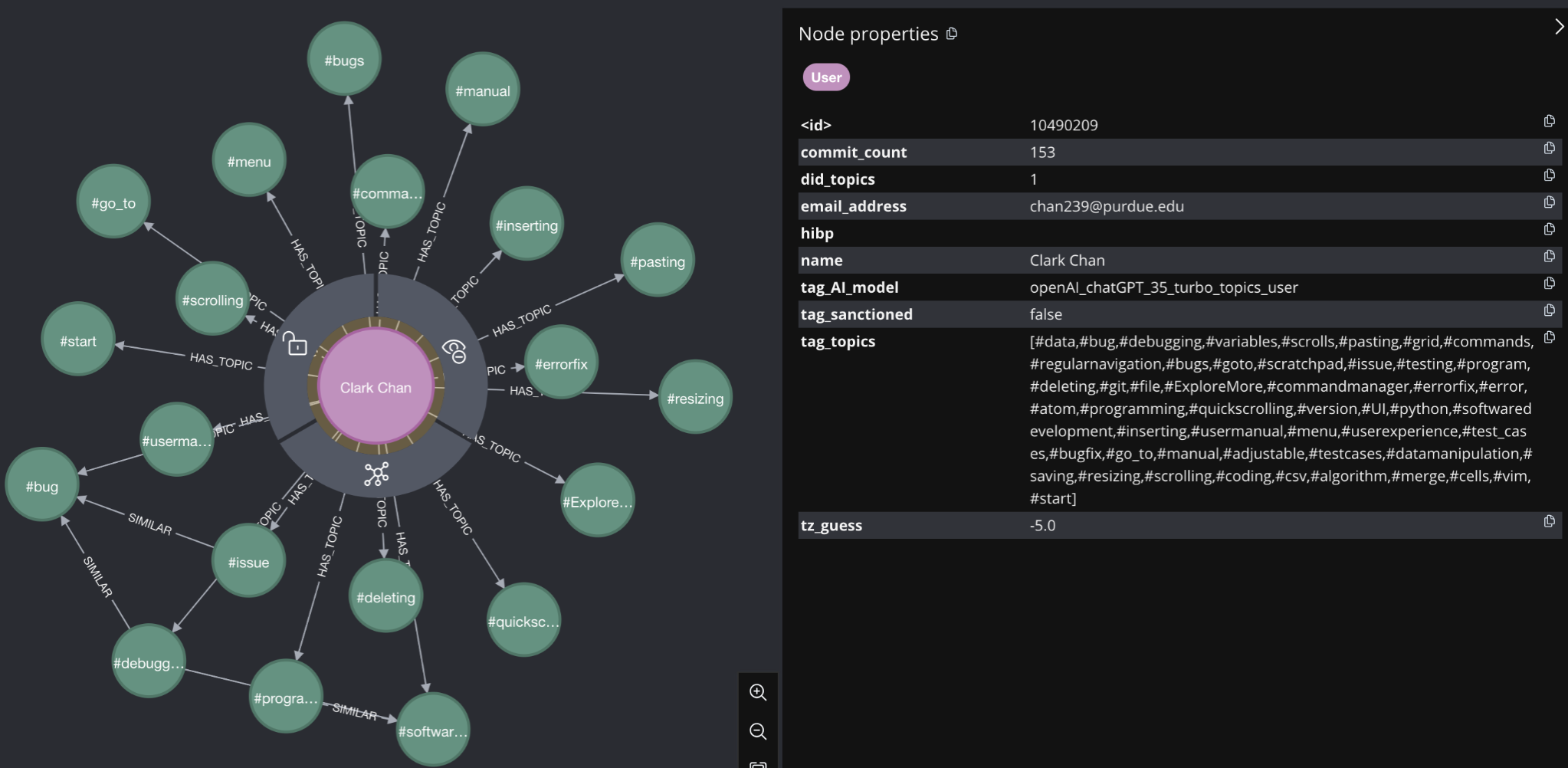
Two: As discussed previously, we use ChatGPT and other LLMs to create Topics (reminder: hashtags)  that describe a User and Repo’s work. These topics are stored in User and Repo nodes as a property. Each topic in a User.topic list is also split out into its own Topic node, with a :HAS_TOPIC relationship pointing from a User to the Topic node. That may be hard to understand - see below! he User node in pink is :HAS_TOPIC related to Topic nodes in green. These topics are also listed in the “tag_topics” property of the User node, highlighted on the right hand side of the screen shot. This distinction is important. The creation of Topic nodes allows us to capture graph structure as a feature to input into our ML pipeline. The topics as a property allow us to run string embeddings on the actual words that make up the hashtags, creating a second, different feature to feed into our training pipeline.

Now that we’ve reviewed some of the important ideas that are fundamental to our work, we can walk through ML efforts, and how we were able to produce results.

Goal: Conduct Entity Resolution on a subproblem within the Reagent Graph Database. This problem is quite large and as a first step to accomplishing it, we define a smaller, more manageable subproblem. Our efforts on this subproblem define the rest of this post. We define our subproblem to be: Use a Link Prediction ML model to correctly identify when two Users have the same name. In plain english - we want a Neo4j ML model to detect when two users have the same name, without explicitly using the name property.

Method: In order accomplish our goal, we executed the following steps:

1. Select ML Type
2. Conduct Data Preprocessing
    2a. Create True Positive Test Cases
    2b. Create String Embeddings
3. Create a Graph Projection
4. Create FastRP Embeddings
5. Create Training Pipeline
    5a. Add Features
    5b. Configure Test/Train split
    5c. Select ML algorithms to use
6. Train the Model
7. Make Predictions
   

1. Select ML Type - Neo4j offers two types of ML algorithms out-of-the-box for usage in graph data science (GDS): Node Classification, and Link Prediction. In order to identify users with the same name, we use link prediction (LP). This is because users with the same name will have a relationship between them specifying this attribute. In the context of our problem, LP predicts where a specific link should exist between two nodes, and doesn’t already exist.

If we have lots of users with the same name, and all but one set of those nodes have a SAME_NAME relationship between them, then a trained LP model will correctly predict that there should be a SAME_NAME link between the two nodes who have the same name, but no relationship between them.

2. Conduct Data Preprocessing - Once we project a graph in-memory (step 3), it is much harder to work with and generally uneditable. Therefore, much of the information we want to include in the graph projection must be made available before we project. In our case, we need to ensure we define our true positive test cases, and turn our node string properties into string embeddings, which are a usable property type in Neo4j projected graphs.

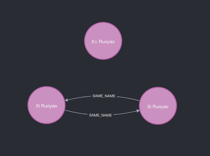
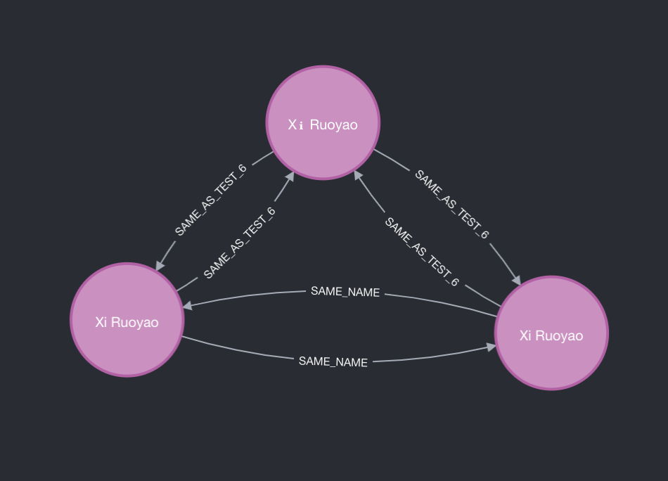
2A. Identify True Positive Test Cases - True positive test cases for our problem are SAME_NAME relationships between two user nodes with the same name. This is easy enough to produce, and we created these relationships for all users connected to the Linux Repo node. However, in order to ensure we had nodes left to predict on, we opted to not toLower() all the name values. This means that, “John Smith” and “john smith” do not have the same name relationship. Further, “Johnny Smith” would also miss the :SAME_NAME relationship. This is exactly what we want, since we now have many true positives (users with the exact same name), and unidentified positives (users with name variations), which we can try and link predict for. Below is a depiction of this:

2B. Create String Embeddings - Because the only node properties allowed in the graph projection are of type float or list of float, we need a way to convert any relevant string properties in our nodes into arrays of floats and store them in their respective nodes. We don’t want to leave this key data out, so we use a popular technique called string embeddings to convert these strings into lists of floats. The theory behind string embeddings is complex, and detailed explanations can be found elsewhere on the internet. There are a few key things to know about them, however:

• String embeddings convert a word, name, or sentence into an array of floats
• The length of the array may be user-specified, but in general, the longer the embedding array, the more precise the float description is.
• We can use measures of “similarity” or “distance” between two embedding arrays to see how similar or close the two vectors are.
• Words, names, and sentences that are similar will have similar string embeddings
  

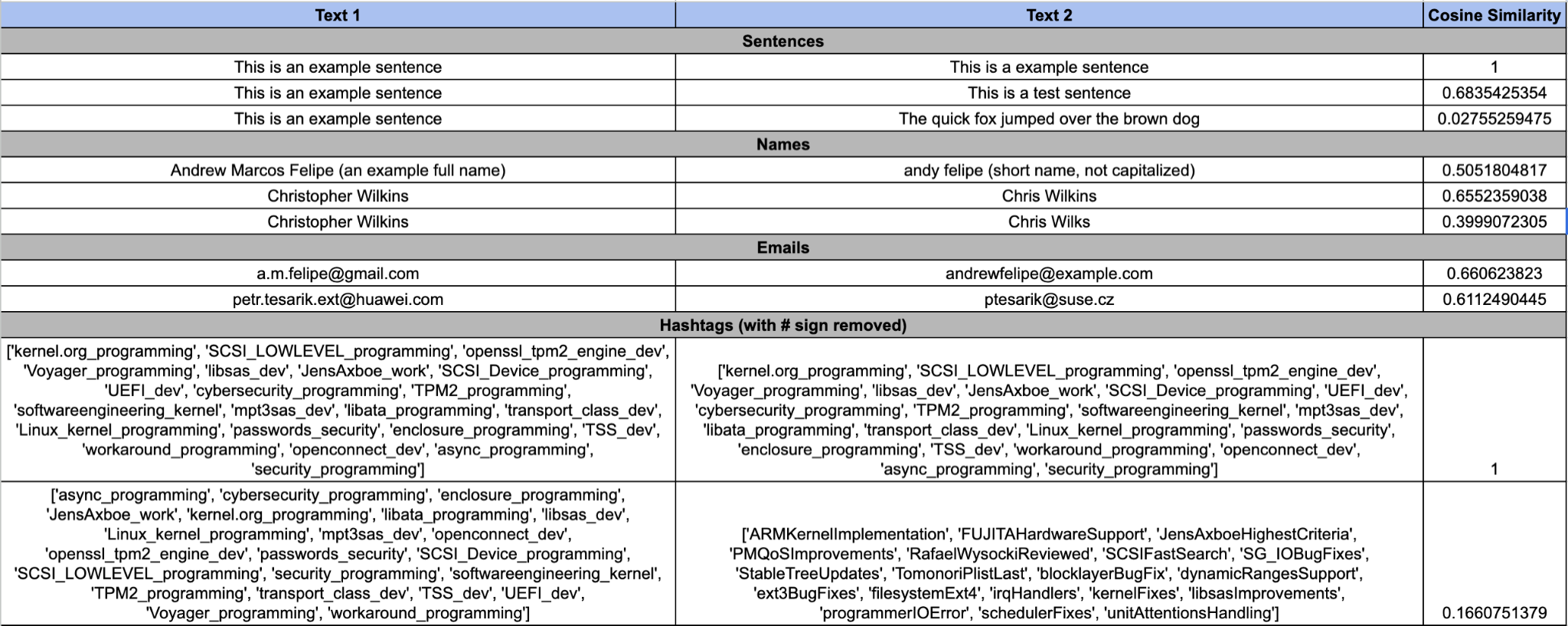
Some examples of this are listed below, where we use a common measure of vector similarity called, “Cosine Similarity” is used to determine the closeness of two float arrays:

We use this string embedding technique to create embeddings for various node properties.

User node: name, email_address, topic_list.

Topic node: name/topic,

Repo Node (only one: linux): name, email_address, topic_list.

These string embeddings are extremely important because they capture node properties that would otherwise be left out of our ML pipeline. When we go to train our graph, they can be used to create input features as measures of similarity between two nodes.

3. Create a Graph Projection - Our graph as a whole is too large to train on, and in its normal format isn’t optimized to do data science with. Neo4j has a special feature that solves both these problems in the graph data science (GDS) library - a projected graph. A projected graph allows us to select a subset of nodes and relationships from our main graph, and only includes node and edge properties that are of type: float or list of floats. The graph projection is kept in-memory and has special properties that allow graph algorithms and special data science methods to be run on it at high speed. Any AI/ML work has to be done on a projected graph in neo4j.

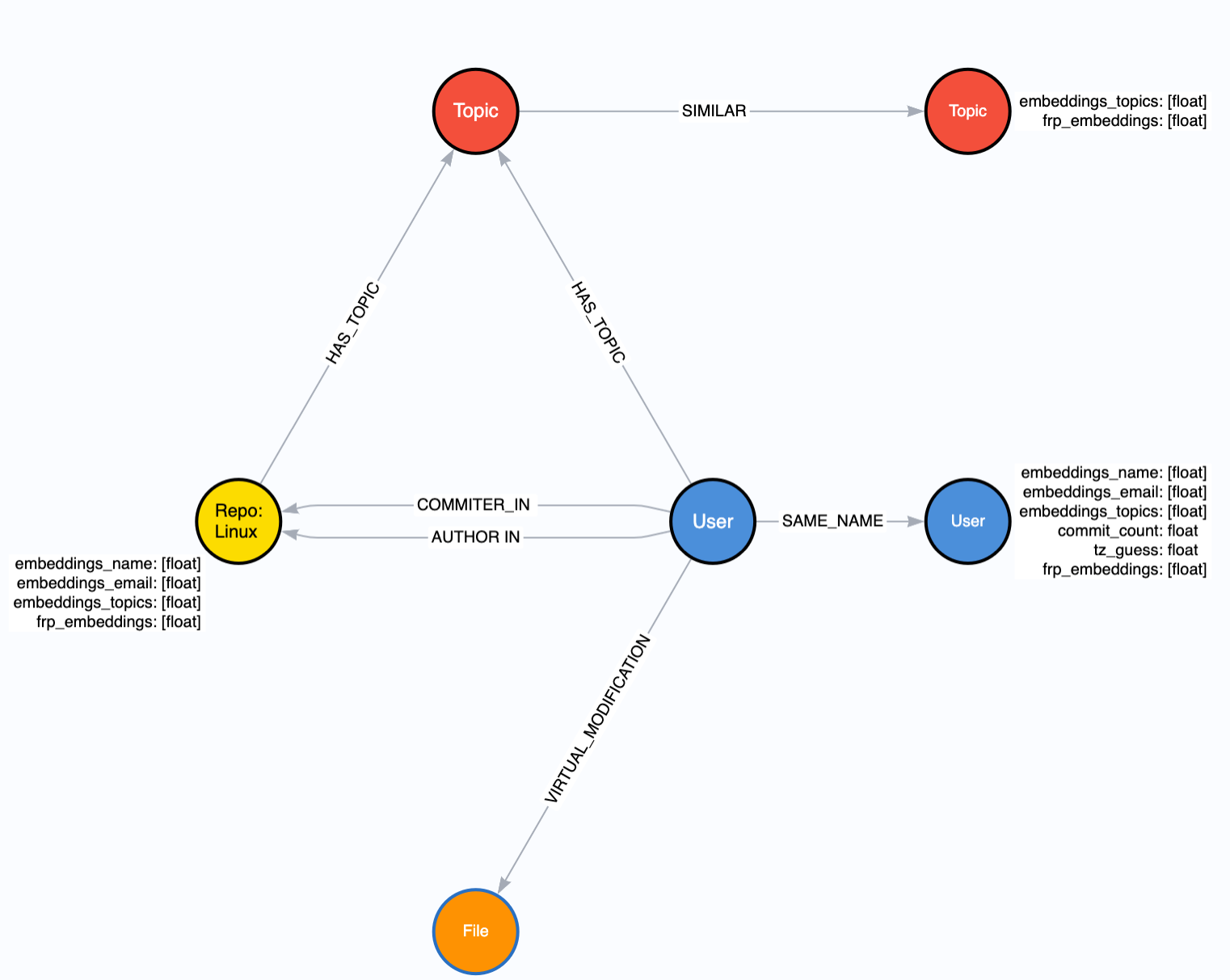
We decided that the best subgraph to project was the graph revolving around the Linux Kernel. We included in our graph the Linux Repo node, any User nodes who have COMMITTER_IN or AUTHOR_IN relationships to the Linux Repo, the Topic (hashtag) nodes associated with the previously listed nodes, and the File nodes that are modified by Users when they commit to the Repo. We use a special kind of relationship between User nodes and Files nodes called a “virtual relationship” - which is basically a temporary relationship that only exists in our projected graph, but not the main graph. A schema of our projected graph can be seen below, including the relevant node properties that will be discussed further on.

The graph projection may have been the most difficult step to complete during the project. While Neo4j offers three separate ways to do graph projection, the documentation for each generally only covers toy problems. We ended up using the cypher aggregation method with a lot of UNION statements. The blogpost by Tomaz Bratanic here was incredibly useful.

4. Create Fast Random Projection (FRP) Embeddings - After projecting a graph to make an in-memory graph, we now have the ability to run additional graph algorithms on our projected graph. One of the most powerful of these algorithms is Fast Random Projections, otherwise known as FRP embeddings. While string embeddings capture node properties as a vector of floats, FRP embeddings capture graph structure as a vector of floats. Again, this is a somewhat complex idea, and won’t be described in depth here, but the important thing to know is that two nodes that have similar neighborhoods of nodes and edges surrounding them will have similar FRP embeddings. So if two user nodes contribute to the same files, have similar topics attached to them, and are both linked to the Linux node, then they will have similar FRP embeddings.

5. Create the Training Pipeline - Now that our graph is projected and has captured data from our string properties, graph structure, and other float properties, we’re ready to build our training pipeline. Neo4j makes this relatively easy with Graph, Pipeline, and Model objects. This means that our graph is separate from the ML pipeline, and the final model is separate from both the Graph and Pipe. This allows us to reuse pipelines on slightly different graphs, and use different pipes on the same graph, all producing individual models that we can evaluate separately.

5A. Add Features - Neo4j currently supports L2 Distance, Cosine Similarity, and Hadamard Product as input features to an ML pipeline. We selected L2 and Cosine for our purposes. These can be reviewed in detail with a quick google or chatGPT query, but it’s important to know here they each of these does some mathematical operation on two input vectors, in our case, the embeddings we’ve created, and outputs measure of similarity or closeness, which the model can train on. We include frp_embedding, embeddings_topics, emeddings_email, timezone_guess, commit_count, and occasionally, embeddings_name.

5B. Configure Test/Train Split - The graph we projected will be broken down into multiple subgraphs each completely disparate from each other. This is surprisingly hard to wrap one’s head around at first, but once it clicks, it’s not too hard to understand. We won’t go too in-depth here. What’s important to know is that a subgraph of our projected graph will be selected to train on. Another subgraph from our projected graph will be used to test the models. And a third feature-input graph will also be created to calculate features.

5C. Select ML Algorithms to Use - Neo4j supports Linear Regression, Random Forest, and Multilayer Perceptron algorithms in their ML pipelines. Since our graph was small enough and we had the time, we opted to use all three. Each algorithm is used to train on the input features, and then tested for performance against the test subgraph. The winning algorithm is returned with its tuned parameters as the ML model.

6. Train the Model - The actual model training portion is rather easy and just takes one call to train the pipeline. The rest of the steps mentioned above: creating a test split, creating a train split, calculating the input features and storing them, training the ML algorithms, testing against the test split, tuning the parameters, retraining, and selecting the winning model, all happen under the hood. This is definitely one of the big perks of using Neo4j!

7. Make Predictions - Once training is complete we can use our trained model to actually make predictions back to our projected graph. We are able to specify how many missing links should be created in our projected graph, and if there is a threshold for the probability assigned to that link prediction being correct. This process, unless otherwise specified, is exhaustive. This means it compares every set of nodes in the graph for missing links. It takes just as long as the training portion. When complete, we’re able to write our relationships back to the main graph and view our results first hand.

Results:

 Before discussing results, it’s important to quickly review exactly what our team did. Many people have done ER, and used ML to do it. Graph databases lend themselves quite nicely to both tasks. What our team has done, which is novel, is:

1. Try to do ER with actors across different projects.
2. Use AI to classify User and Repository data with topics (hashtags), turn these topics into both node properties and nodes themselves, create string embeddings and FRP embeddings out of the topics (and other nodes), and include them in an ML pipeline as a feature.
   

 With limited success we were able to predict the missing :SAME_NAME links. The majority of our ML runs did not correctly predict missing links. However, we feel that the method introduced here can be successful with more work. Below is a result from one of our successful runs. It should be noted that this ML run did include the actual embeddings_name property, which is a proxy for name itself. However, we feel confident that this method of ER can and will be more successful in the future.

 Challenges: Our biggest challenge here is the precision of topics created by our LLMs. The LLMs we used are impressive and do a good job of creating hashtags for user and repo data. However, they are oftentimes too general. . The same data presented twice could produce different hashtags with high variability. Further, they often times don't reach the level of granularity that is helpful in this kind of problem. Instead of producing Topics of user such as: #Linux #Programmer, it's much better to have Topics: #BootLoaderDev #UEFI. This more precise tags allow us to better approximate how similar two user's bodies of work are. This problem may recede in the future as LLMs get better at their work, but it's also an issue of data availability. The better, more descriptive data we have for a user or repo node, the more precise it's topics will be.

 Future Work: Ideally we’re able to correctly predict without the embeddings_name property, however our successful runs all included this property. This makes sense, since two name embeddings will have very similar vectors. In the future we will strive to achieve success without this embedding.